Update articlev1.1.02026.11.02

Motors without magnets, from a specification: SynRM and SR design, efficiency maps, slide and Excel reports

Initial design of induction, SynRM, wound-field and SR motors from a specification, side-by-side efficiency maps, JMAG-RT model export, slide and Excel reports, memory across conversations and in-app help, shown with the actual screens and prompts.

See all changes

Play update video

Playing the video is subject to YouTube's privacy policy.

v1.1.0 widens the range of motors that can go from a specification to an initial design and analysis. Squirrel-cage induction motors, SynRMs, wound-field synchronous machines, axial flux motors and SR motors now follow the same flow as PMSMs. For comparing designs there are side-by-side and difference efficiency maps; as the way out of a design there are JMAG-RT model export and slide and Excel reports. In the app, the AI remembers instructions across conversations and answers questions about how to use the app.

Design featuresInitial design for induction, SynRM, and wound-field machines; axial flux and SR motor analysis; efficiency map comparisons; JMAG-RT model export; MATLAB / Simulink integration; PLECS circuit simulation integration

ReportsSlide-format reports, Excel reports

The app and usabilityMemory across conversations, ask about the app in chat, selectable installation folder, about this app

Initial design for induction, SynRM, and wound-field machines (video 0:25)

Squirrel-cage induction motors, SynRMs and wound-field synchronous machines (WFSM / EESM) can now be designed and analysed from a specification document in the same flow as PMSMs: sorting the requirements, candidates for the template and the pole and slot numbers, an analysis plan, then building and analysing after approval and checking the target points with FEM. When the specification cannot be met, the process stops and reports the reasons with numbers. The video takes a SynRM, which has no magnets, through three requests.

The specification is a JSON file: 4 poles and 24 slots, a stator outer diameter of 204 mm, an air gap of 1.0 mm, a stack length of at most 100 mm, inverter limits of 380 Vrms line voltage, 40 Arms phase current and 4500 rpm, and three target operating points: 30 Nm at 1500 rpm, 20 Nm at 3000 rpm and 8 Nm at 4500 rpm.

The first request asks for the sorted requirements and the candidates. Nothing is run yet; the plan is approved after reading it.

From the specification in @spec_synrm.json , make an initial design of a synchronous reluctance motor (no magnets).
Sort the requirements, show the candidates (poles, slots, template) with your reasons, then present the analysis plan (case count and expected duration) and wait for my approval. Do not run anything yet.
A parallel solver licence (PSL, 64 jobs) is available. Template defaults are fine for materials the spec does not give. Name the file synrm_4p24s.jproj.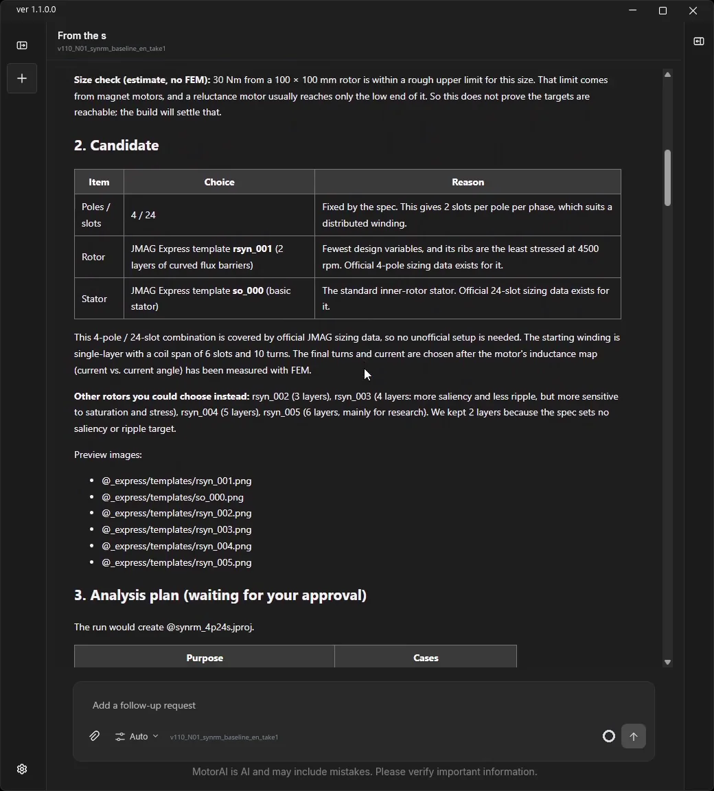

Table of sorted requirements, the recommended SynRM template and the main dimensions — The requirements are sorted into fixed values, limits and constraints, and a recommended and an alternative SynRM template from JMAG Express are shown with reasons. Because a SynRM has no magnet-induced voltage, the plan says the number of turns is decided by analysis rather than on paper

The plan is up to 36 cases in about 17 minutes: one reference point, a 24-case grid of current and current angle to identify the dq model, two checks after the turns are fixed, the three target points, and six correction cases used only if a target falls short.

The second request approves the plan and allows up to two corrections if a target point falls short. The figure format is also specified here.

Go ahead with the plan and run all the cases you proposed. If a target point falls short you may correct up to twice and re-analyse; those extra cases are approved too. When done, show the table of target / prediction / FEM / source and a single scatter plot of torque against speed (required and analysed values as markers only, never joined by lines, each point labelled with its speed, title on one line). Give the saliency ratio and power factor per operating point. Show only that scatter plot and one cross-section image of the built model in the reply.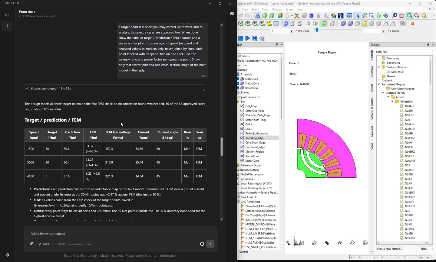

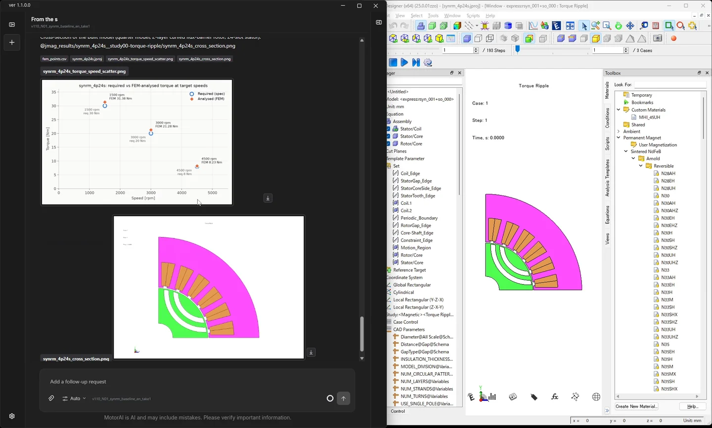
Comparison table of target, prediction and FEM, and the saliency ratio and power factor per operating point, with the SynRM model in JMAG-Designer on the right — All three targets were met on the first FEM check, so no correction round was used: 30 cases in about 12.5 minutes. The reply states 11 turns per coil and a current density of 5.23 A/mm², and notes that the saliency ratio and power factor come from the inductance map rather than from a direct measurement

Scatter plot of required and analysed torque, and the cross-section of the built model — As requested, only two figures are shown: the scatter plot and the cross-section. The FEM torque exceeds the targets by 2.8 to 6.4 %, and the line voltage and current stay inside the limits at every point

The third request checks whether any analysis is still waiting for approval. This time nothing was left, so only the final table and figure come back.

If any analysis is still waiting for my approval, run all the cases you listed as they are. When it is done, show the final comparison table and the single scatter figure.

Axial flux and SR motor analysis (video 1:56)

For axial flux motors (1 rotor 2 stators / 2 rotors 1 stator) and SR motors you can now go from a specification through model creation, the number of turns, analysis and a report in a single conversation. If the specification is ambiguous or the configuration is not supported, the process stops with the reason. The video builds and analyses a 6/4 three-phase SR motor in two requests.

The first request sorts the specification and builds the model. It asks the AI to raise only the points that need confirming and not to run any analysis yet. In this recording nothing needed asking, so the model was built straight away; when something is unclear, a question card appears first.

I want to build and analyse an SR motor from the specification below. First sort the spec, propose candidates, and ask only what needs confirming. In this turn stop after building the model; do not run any analysis yet.
Machine: switched reluctance motor (SRM), 3-phase, 6 stator poles / 4 rotor poles
Stator outer diameter 70 mm, stack length 80 mm
DC voltage 45 V, current limit 45 A (phase current peak)
Speed 10000 rpm, target torque 0.5 Nm
Template defaults are fine for anything not specified. Name the file srm_6_4.jproj, and show one cross-section image of the built model.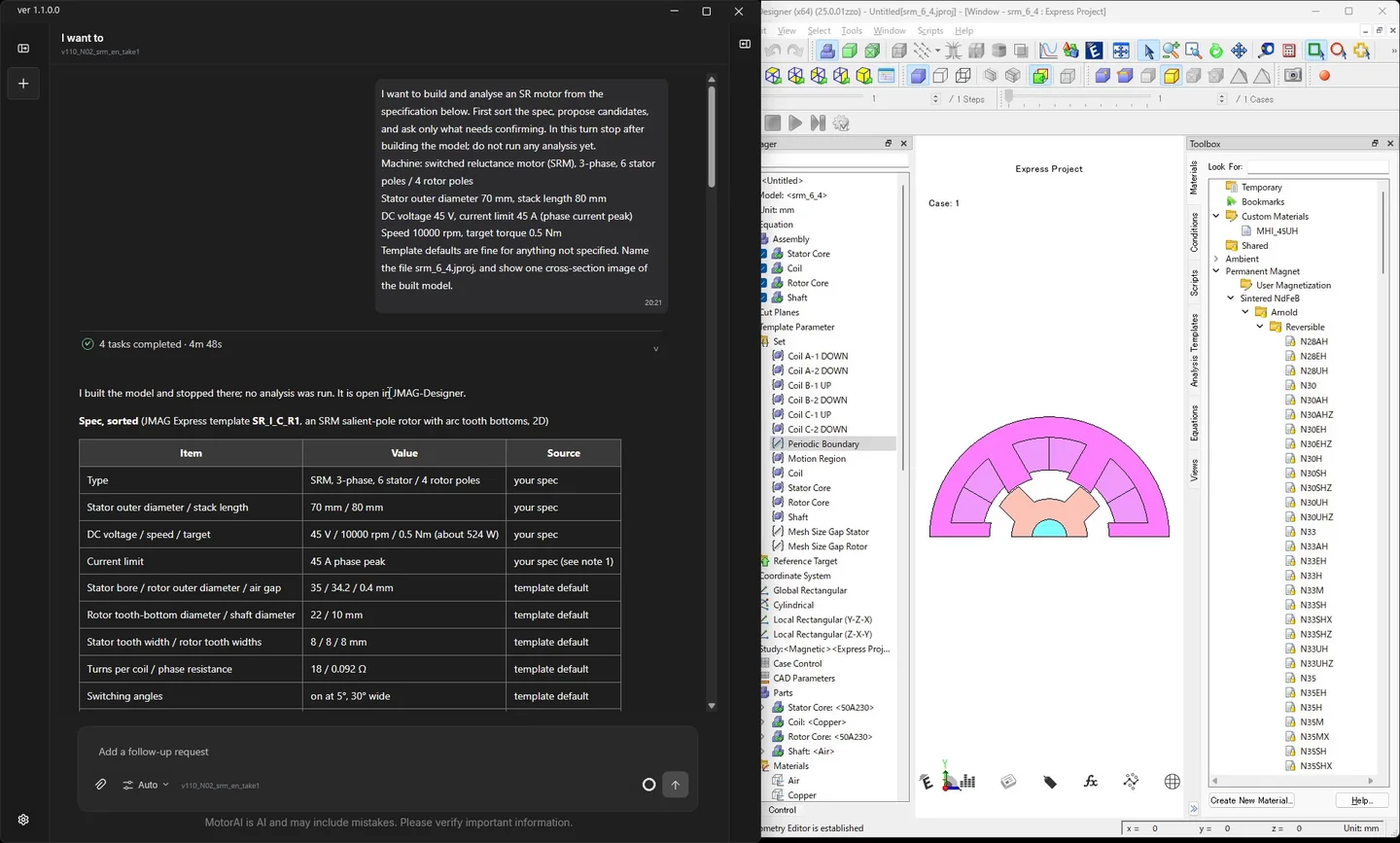

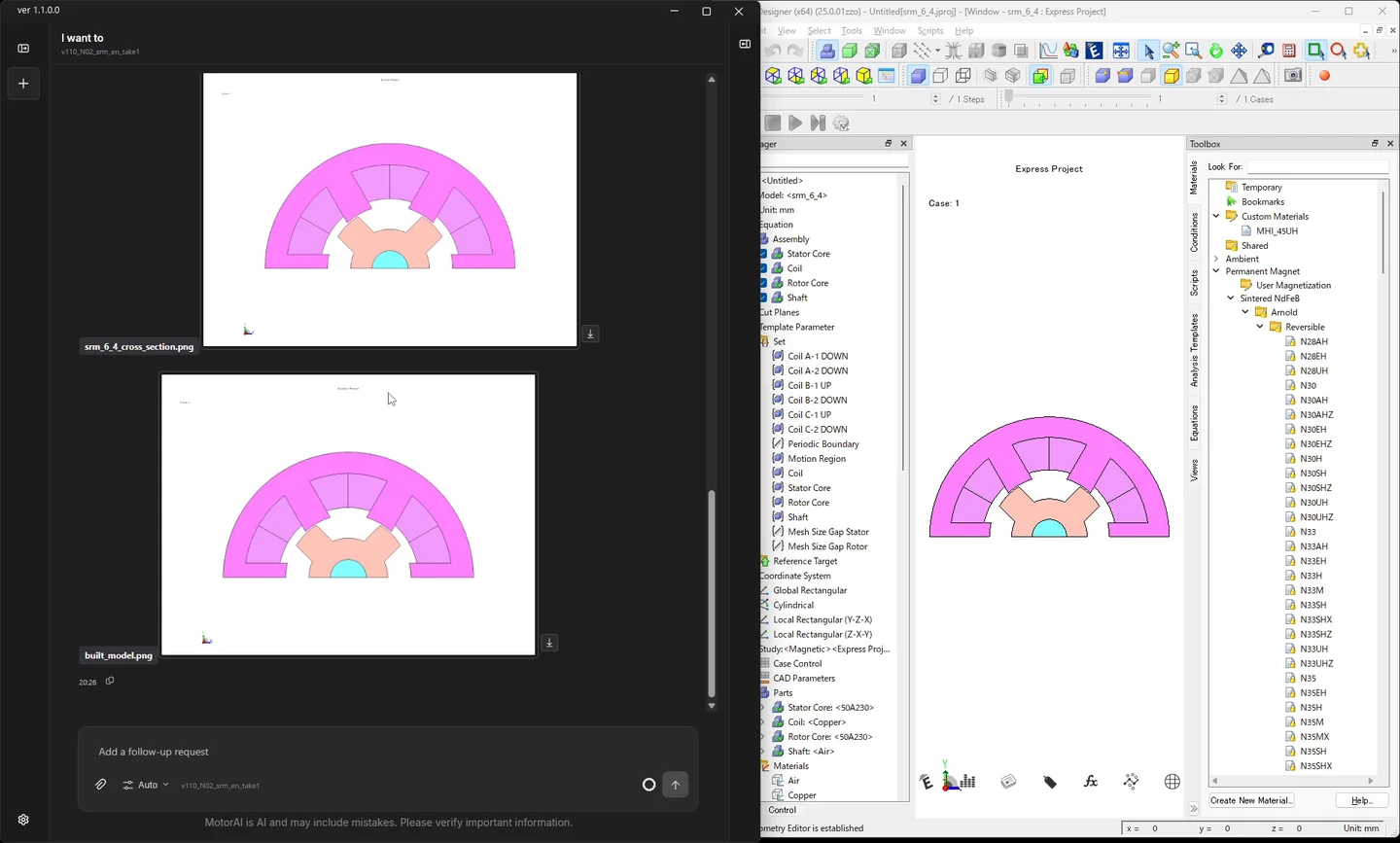
The sorted specification with the value of each item and where it came from, and the candidate configurations — Each item is listed with its source: the specification or a template default. The 6/4 configuration is kept, and a 12/8 alternative is described with its trade-offs

Cross-section of the built SR motor, with the model open in JMAG-Designer on the right — The 6/4 model is built with the template defaults for the undefined items (18 turns, switching on at 5° for 30°, a 0.4 mm air gap, the materials) and opened in JMAG-Designer

The second request decides the turns and runs the load analysis. The approved case count is given as a number, and the items for the result table are listed.

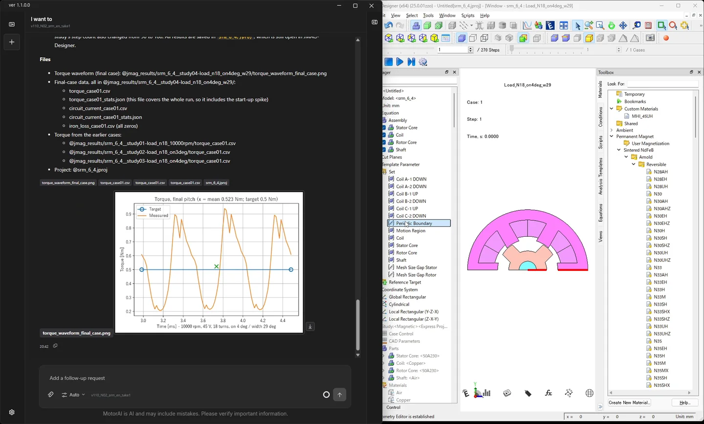
Decide the number of turns with an excitation probe, apply it, and run the load analysis. I approve 2 cases in total (1 sizing case + 1 main case), plus up to 3 more cases if a correction is needed. Report average torque, torque ripple, copper loss and iron loss in a table, the drive conditions used (voltage, conduction angles), and which items are verified or not. Show exactly one torque waveform figure.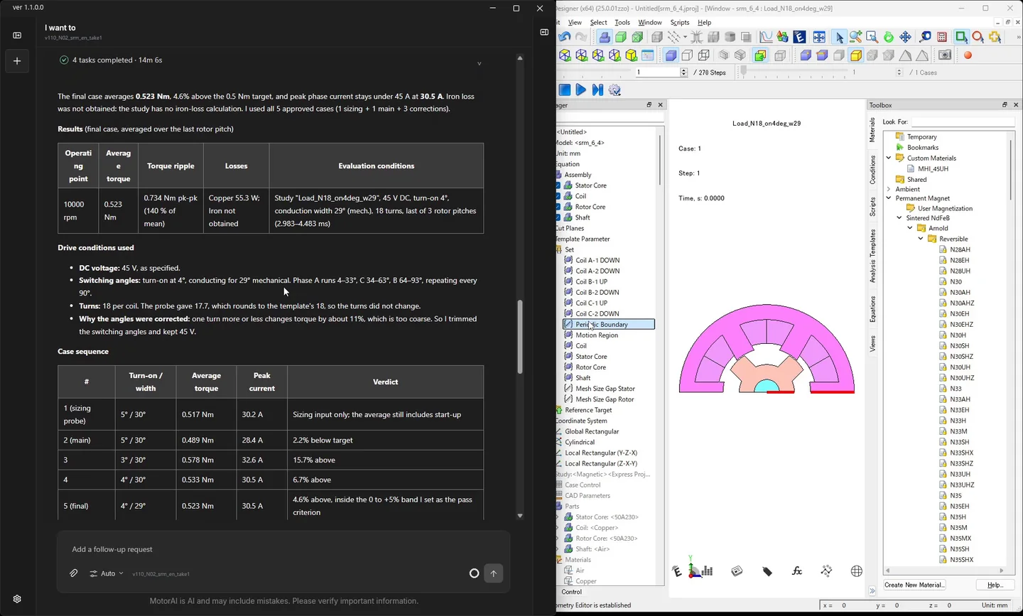

Table of average torque, torque ripple, losses and evaluation conditions, with the verified and unverified items — The probe confirmed 18 turns. The first load case gave 0.489 Nm, 2.2 % short of the target, so the AI trimmed the switching angles within the approved cases and reached 0.523 Nm (+4.6 %) with a peak current of 30.5 A. The iron loss could not be obtained because the study has no iron-loss calculation, and the table says so

Torque waveform of the final case, with the list of result files above it — The waveform of the final case is shown with the 0.5 Nm target line. Above it, the reply lists the five cases with their switching angles, torque and peak current; each correction run was approved on an approval card before it started

Efficiency map comparisons (video 3:28)

Side-by-side efficiency maps of several designs, and difference maps of efficiency, total loss, copper loss and iron loss against a baseline design, can now be made from chat. Starting from a baseline design A whose efficiency map already exists, the video makes a design B with a 30 % thinner magnet, computes its efficiency map under the same conditions, and compares the two.

The first request creates design B and computes its efficiency map. The conditions for the dq-parameter map and the efficiency map are written out so that they match design A.

d-model_base.jproj in the working folder is the baseline design A, and its efficiency map is under maps/design_a/. Make a copy design_b.jproj yourself (do not ask me) and turn it into design B by reducing the magnet-thickness variable in the design table by 30 % (if the geometry safety check stops you, write the design-table value directly and continue). Do not change the original file.
For design B, measure the dq parameter map and compute the efficiency map under the same conditions as design A: current amplitudes 0, 4.24 and 7.07 A (0, 3 and 5 A rms; 0 A is the no-load reference), phases 0 to 90 degrees from the q axis in 10-degree steps, the speed as set in the study, and add any probe you need. Use PSL (64 jobs) and run without waiting for my confirmation, case count included.
The efficiency map uses 165 V DC, space-vector PWM, the measured current limit, the model's phase resistance, shaft torque with the iron loss taken from the shaft output, 500 to 6000 rpm on linear axes. Save the figures under maps/design_b/ and show only the efficiency map in the reply.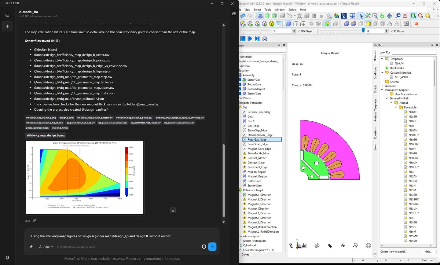

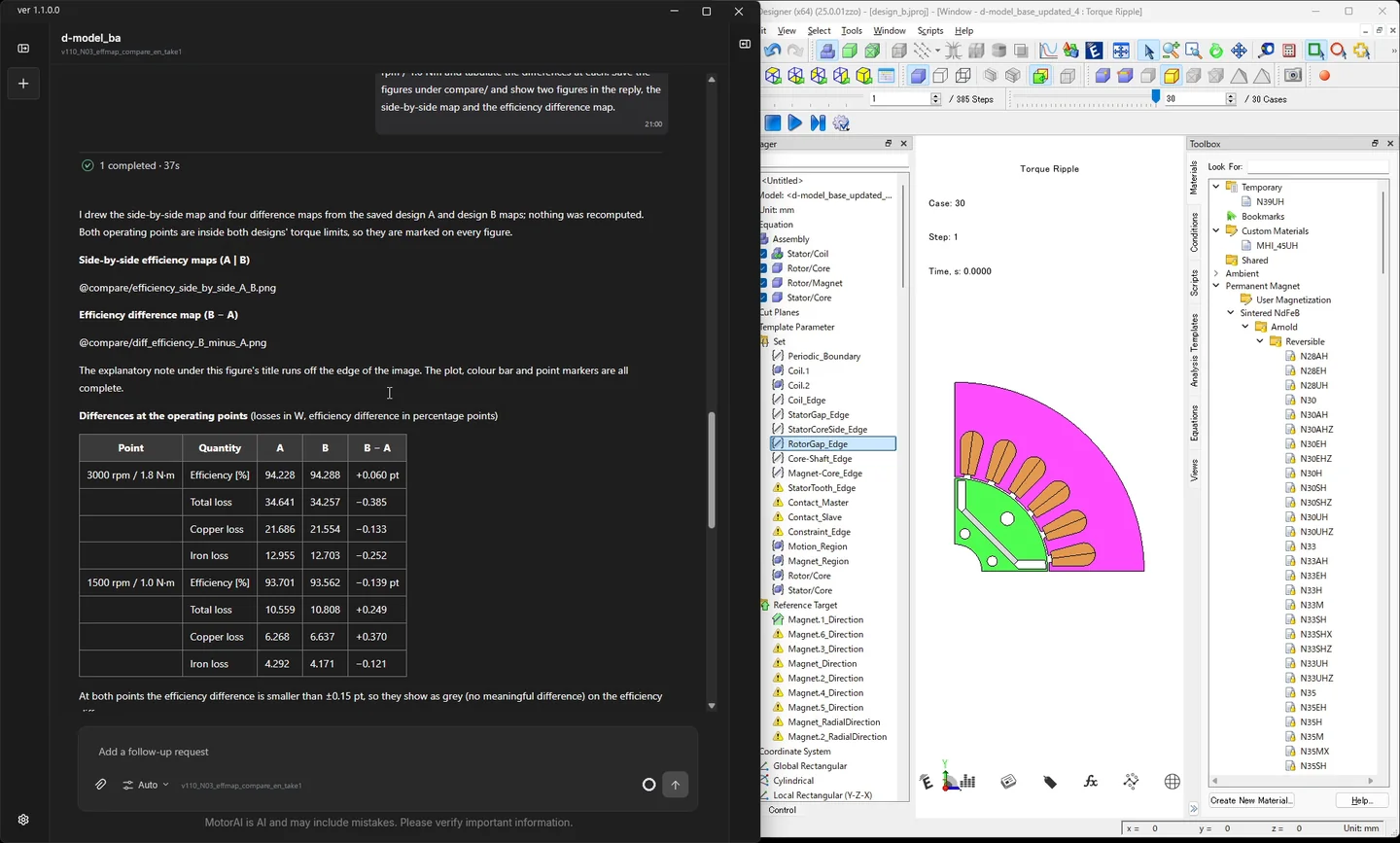
Efficiency map of design B, with the design B model open in JMAG-Designer on the right — The magnet-thickness variable was changed from 2.5 mm to 1.75 mm in a copy, 33 cases were solved in 265 s, and the efficiency map was drawn. The reply confirms that the original file was not changed

The second request draws the comparison figures. They are drawn from the existing figures, so nothing is recomputed.

Using the efficiency-map figures of design A (under maps/design_a/) and design B, without recomputing, draw the side-by-side efficiency maps and the difference maps of efficiency, total loss, copper loss and iron loss against design A. Mark the operating points 3000 rpm / 1.8 Nm and 1500 rpm / 1.0 Nm and tabulate the differences at each. Save the figures under compare/ and show two figures in the reply, the side-by-side map and the efficiency difference map.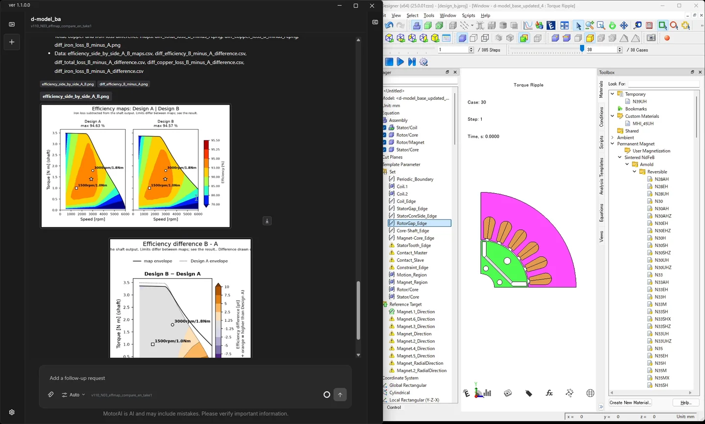

Side-by-side efficiency maps of A and B, and the efficiency difference map — The side-by-side maps share one colour scale. The difference map shows that the thinner magnet of B gains up to 9.6 points at high speed and light load and loses up to 2.5 points at low speed and high torque

Table of the efficiency, total loss, copper loss and iron loss differences at the two operating points — At the two marked points the differences are tabulated: B is 0.06 points more efficient at 3000 rpm / 1.8 Nm and 0.14 points less efficient at 1500 rpm / 1.0 Nm

JMAG-RT model export (video 4:49)

A JMAG-RT model can now be exported from a finished PMSM design, with the no-load flux linkage and the d- and q-axis inductances reported in a table. The video splits this into a plan request and a run request.

d-model_base.jproj in the working folder is the finished design. Export a JMAG-RT model from it; it will be used later for control simulation. The Simulink block file is not needed this time; the RT model file (.rtt) and the characteristic table are enough.
The motor ratings are 165 V DC, 7.07 A maximum current (phase peak, 5 A rms) and 6000 rpm maximum speed. Take the winding of the study "Torque Ripple" as the adopted design. You may use PSL with up to 40 parallel jobs (the scheduler setting, which fits in memory). Show me the plan first.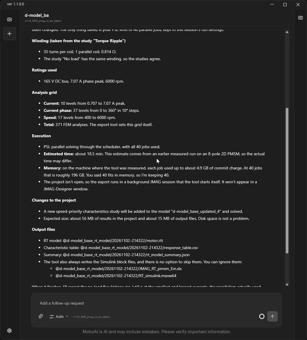

The export plan: the adopted winding, the FEM case count, parallel jobs and expected time, the output folder and notes — The winding (35 turns, 0.814 Ω), the grid of 10 currents × 37 phase angles × 17 speeds (371 FEM cases), 40 parallel jobs and an estimate of about 18.5 minutes are shown before anything runs, together with the output folder and what will change in the project

OK, go ahead with that plan. When it is done, show the no-load flux linkage and the d- and q-axis inductances at the smallest and largest currents in a table, and give the location of the output files.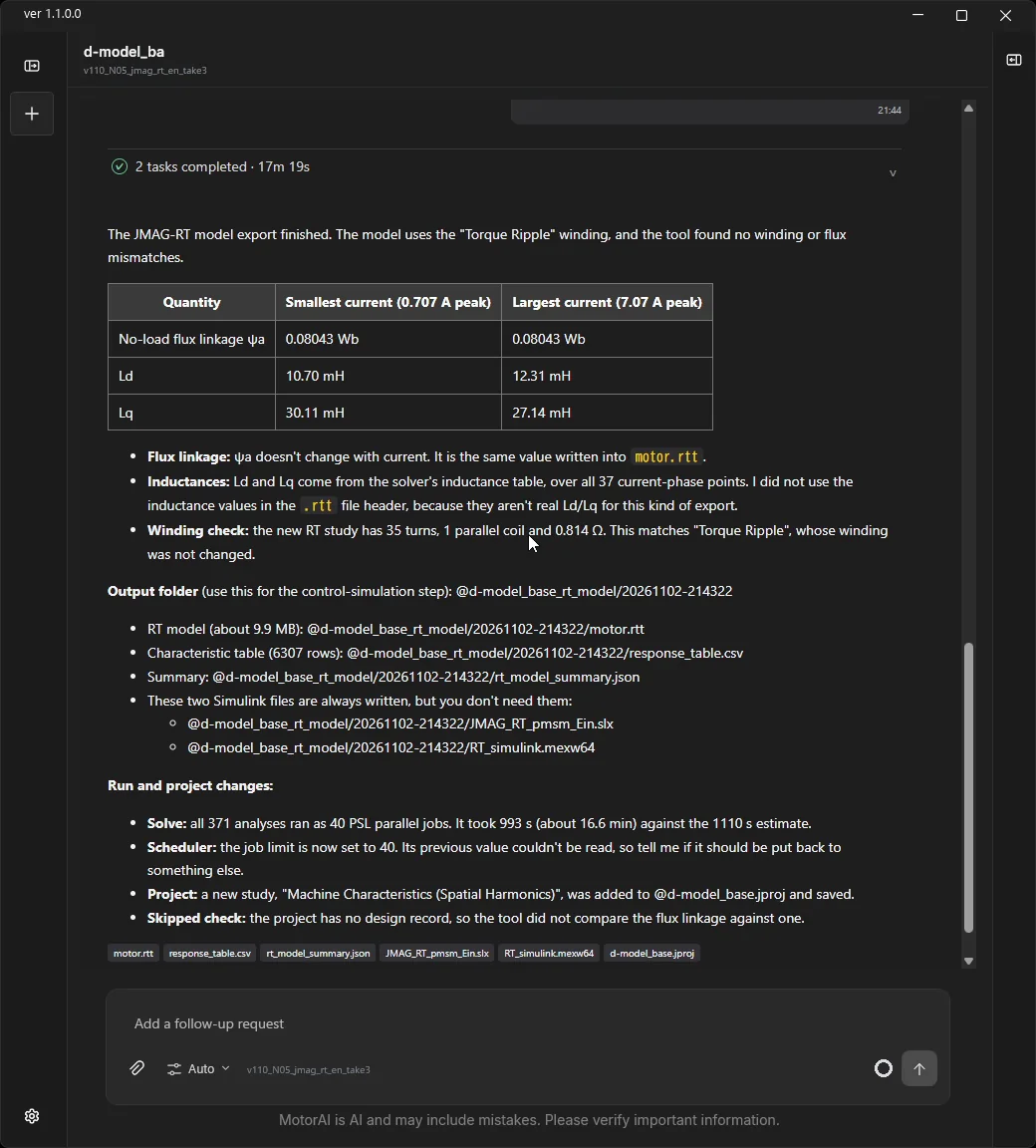

Table of the no-load flux linkage and Ld / Lq at the smallest and largest currents — The 371 cases were solved with 40 parallel jobs. The table gives a no-load flux linkage of 0.0804 Wb, Ld rising from 10.70 mH to 12.31 mH and Lq falling from 30.11 mH to 27.14 mH with current. The reply notes that the Ld / Lq values come from the solver's inductance table, not from the header of the .rtt file

Slide-format reports (video 5:43)

Design and analysis results can now be compiled into a slide-format report (PDF). Reports can hold comparison tables against a baseline design, Pareto charts and cross-section figures, and an editable PowerPoint file is produced on request. You can match the style of your own .pptx / .pdf sample, or use a document-oriented theme with smaller text to fit more on each page.

The video starts with the result of a JMAG multi-objective optimization (MOGA) placed in the working folder. The motor is a 10-pole 12-slot surface permanent magnet motor; the two design variables are the magnet thickness and the tooth width, the objectives are the efficiency at the rated point and the torque ripple, and the constraint is an average torque of at least 95 % of the baseline. The folder holds the result CSV of 144 individuals and cross-section images made from the JMAG model.

The first request sorts out the result. What goes into the report is settled in the conversation before the report is made.

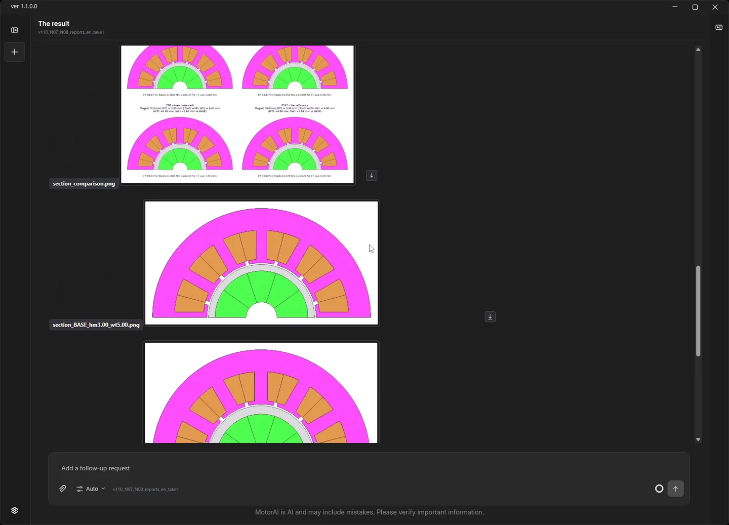
The results folder holds a JMAG multi-objective optimization (MOGA, 144 individuals). Under the conditions in the README, sort out the efficiency / torque-ripple Pareto front among the feasible designs, pick three representatives from the front and compare them with the baseline. Use the images in the sections folder for the cross-sections and state the magnet thickness and tooth width so that it is clear what changed.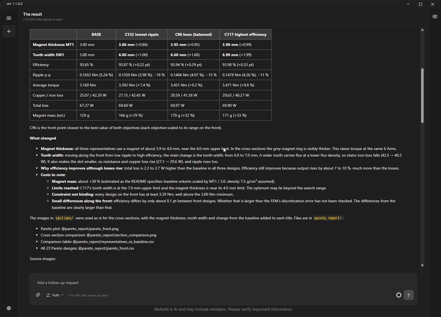

Comparison table of the three representatives and the baseline, and the points read from the result — Of the 139 feasible designs, 23 form the Pareto front, and representatives A, B and C are taken from its ends and its knee. The reply explains that efficiency rises because the output rises rather than because the losses fall, that the magnet thickness sits at the upper limit of the search range, and that the magnet mass grows by about 30 %

Pareto chart and the cross-sections of the baseline and the three representatives — The cross-sections come from the images in the working folder, with the magnet thickness, the tooth width and the change from the baseline written on each

The second request makes the slides. The elements to include and the editable format are asked for.

Compile this into a slide-format report (PDF) with a comparison table against the baseline, the trade-off chart and the cross-sections of the three designs, and also produce an editable PowerPoint file.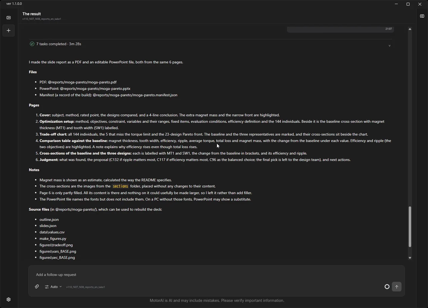

The page structure of the slides and the list of the PDF, PowerPoint and source files — Six pages: a cover with the conclusion, the optimization setup, the trade-off chart with the cross-sections, the comparison table, the cross-sections side by side, and a summary with the open points. The extra magnet mass and the narrow front are highlighted on the cover

In the PowerPoint file the text, tables and flow diagrams stay editable; figures are embedded as images.

Excel reports (video 7:01)

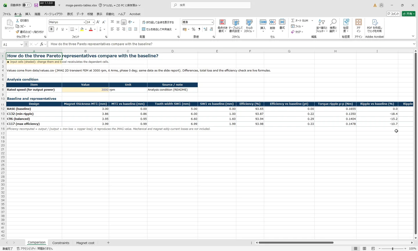
Comparison tables against a baseline, judgements and calculations such as material costs can now be made as Excel workbooks with live formulas, as attachments to a report. The workbook is built from the same numbers as the slides, so the values do not drift apart.

As an attachment to the report, make an Excel workbook with live formulas holding the comparison table against the baseline, the constraint judgements, and the magnet material cost (NdFeB at 15,000 yen per kg).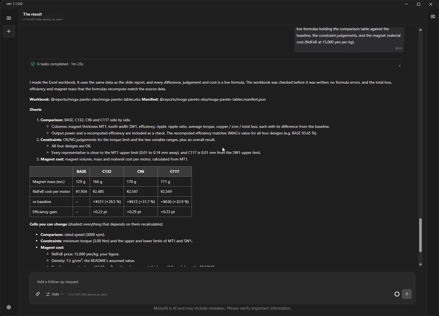

Description of the three sheets of the workbook and the magnet material cost table — Three sheets: comparison, constraints and magnet cost. The material cost is ¥1,934 for the baseline and ¥2,485 to ¥2,569 for the representatives, and the price, density and baseline magnet volume are shaded cells you can change. The reply says that every formula was checked and that the recomputed values match the source data

The comparison sheet opened in Excel — Opened in Excel, the difference and ratio cells hold formulas. Changing the unit price updates the related calculations

Memory across conversations (video 7:38)

What you ask the AI to remember now carries into new conversations. For instructions that affect how future work is done, the AI asks before saving. You can also ask in chat to see or delete what it remembers.

Please remember this. Whenever I ask for a figure, use a linear speed axis in rpm and write the axis labels and legend in English.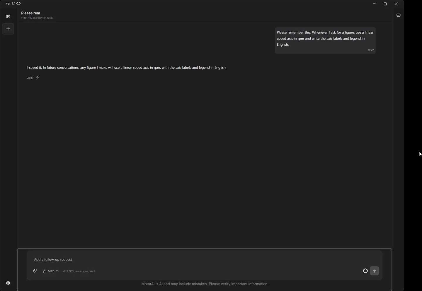

Reply confirming what was remembered and saved — The AI repeats the preference it has saved and says it will apply in later conversations

A new piece of work is started so that the next question is in a different conversation.

What do you remember about me? Show it as a list.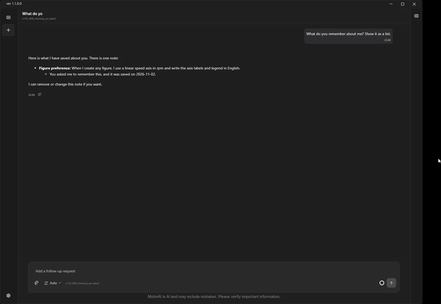

List with the one note from the previous conversation — The note from the previous conversation is listed with the date it was saved and the request that created it

Forget the instruction about the axis labels and legend.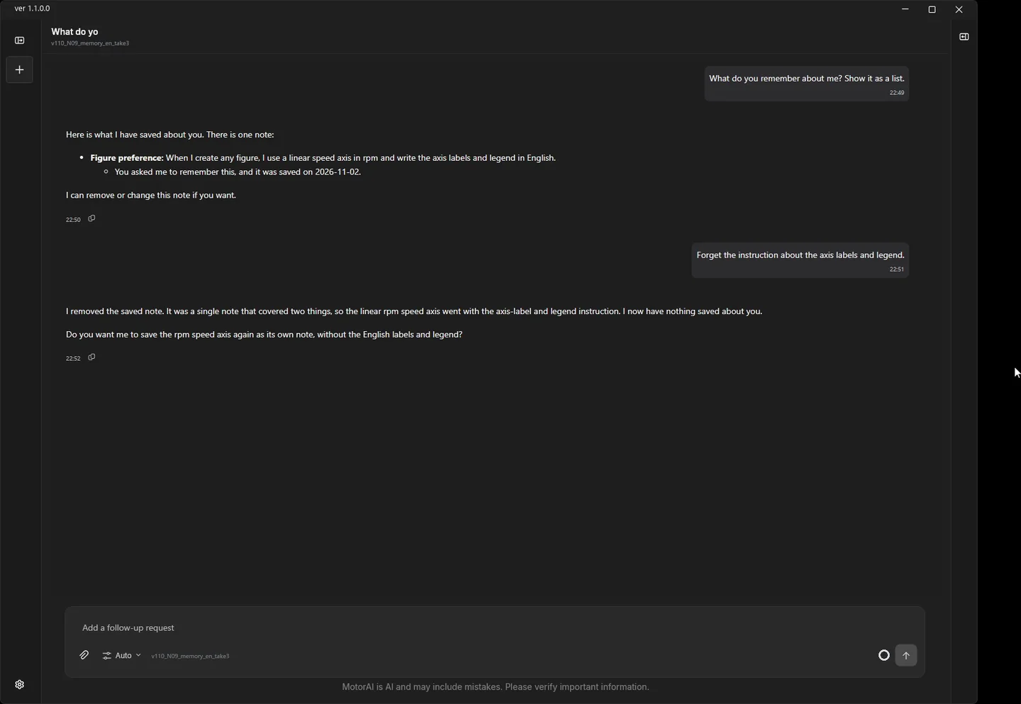

Reply reporting that the note was removed and offering to save the speed-axis part again — Because the two instructions were saved as one note, the AI removes the note and explains that the speed-axis part went with it, then offers to save that part again on its own. In the Japanese recording the same request produced a question card asking how much to forget

Ask about the app in chat (video 8:13)

Questions about how to use a screen, what a setting does, or what to do when something is not working are now answered in chat, tailored to your installed version.

An approval card appears every time I ask for an analysis. I want fewer confirmations. Where do I change the setting?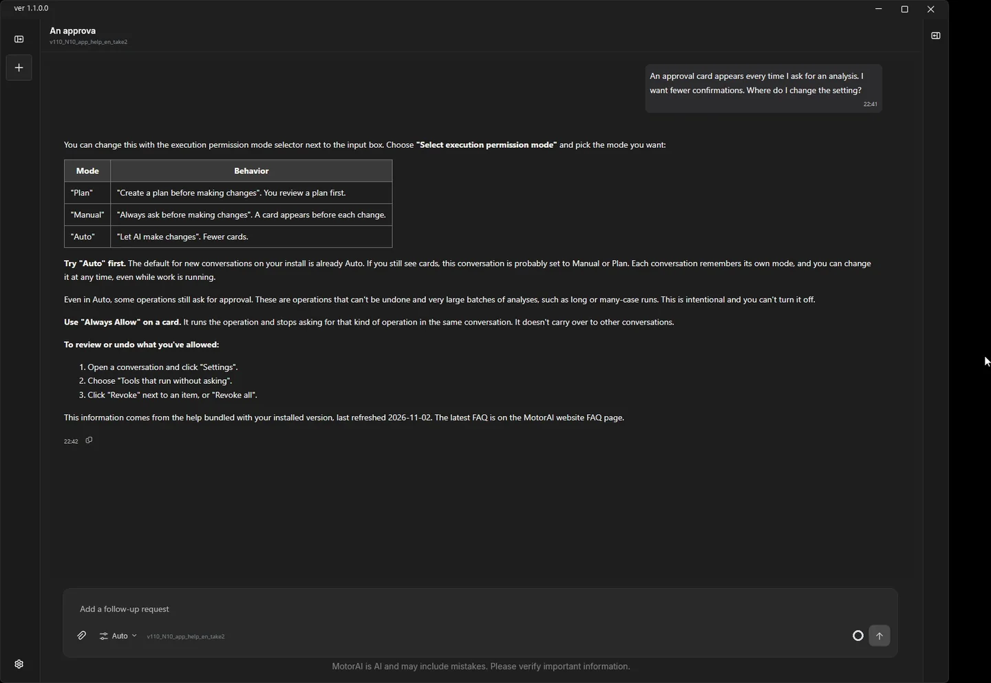

Answer explaining where the permission mode is switched and how "Always allow" works and is revoked — The answer points to the execution permission mode selector next to the input box, suggests Auto, explains that operations that cannot be undone and very large batches still ask, and shows where "Always Allow" is reviewed and revoked in Settings

What should I check when JMAG is not detected?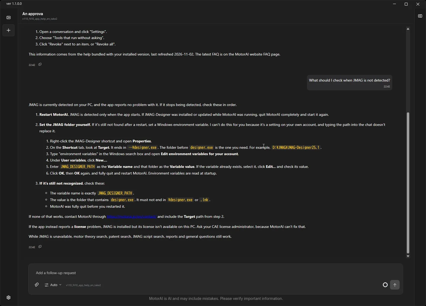

Answer that first checks this PC, then lists the steps to take when JMAG is not detected — The AI first checks this PC and reports that JMAG is detected, then gives the steps for when it is not: restart the app, set the JMAG_DESIGNER_PATH environment variable from the shortcut's target folder, and the points to check after that

About this app (video 8:45)

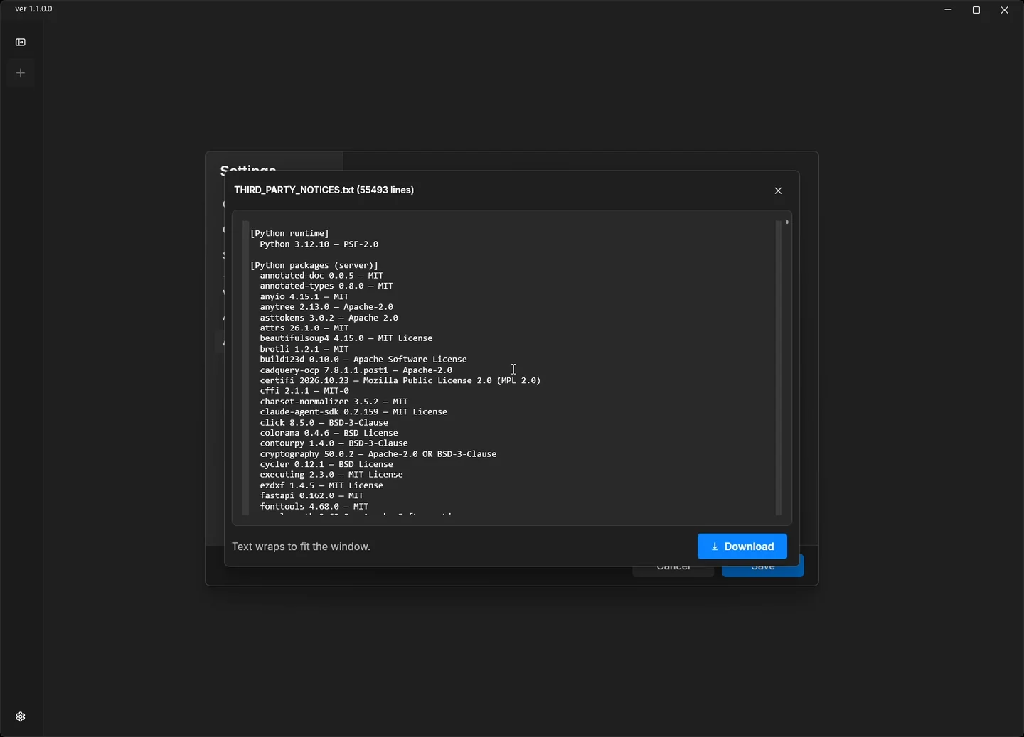
An "About" section has been added to the settings screen, where you can view the licenses of the open-source software included in the app.

The third-party software list opened from About in Settings — The included software and its licenses are listed with the license texts. The text can also be downloaded

Other new features

The following features are also part of v1.1.0 but are not in the video.

MATLAB / Simulink integration: Simulink models can now be explained, edited (block parameters and structure), and simulated with summarized results through chat. You can also search for and import examples shipped with MathWorks products.
PLECS circuit simulation integration: PLECS models can now be explained, edited (component values, circuit topology, control blocks), simulated, and compared through chat. Edits are made on a copy, so your original model is never changed.
Selectable installation folder: The installation folder for the app can now be chosen during installation.

Other improvements and fixes

Improvements:

JMAG-Designer 25.2 is now supported. The app checks which features are available in your JMAG version and adapts its behavior, so it works with both 25.0 and 25.2. The JMAG Express template list now shows only templates available in your installed JMAG.
PMSM initial designs from a specification (IPM / SPM, inner / outer rotor) can now be analyzed with FEM to check whether the target operating points are met, and points that fall short are corrected in the design. If the targets cannot be met, the reasons are reported with numbers along with the range that was explored.
When converting to the JMAG-Express standard structure, magnetization is now set up in the native Express format, and windings that templates cannot represent can also be converted. Rotor and stator grafts can now handle outer rotors, IM bar counts, AFM models of the same configuration, and SR stators.
Geometry Editor equations that have no row in the design table can now be registered as rows and swept.
The AI measures the project file size as it works so that a single project file does not grow too large, and asks whether to move to a new file, clean up unneeded results, or continue when the limit is near. Optimizations no longer save detailed results for each individual by default.
When a specified name is not found in the model, the existing names are suggested. Bulk analyses of 9 or more cases are confirmed through an approval card showing the study name and case count.

Fixes:

Analyses that ignored the requested execution method ("in parallel with PSL", "as a batch") and ran one case at a time, failures when creating a JMAG standard efficiency map study, and speed divisions and maximum speed not applied to the study.
A rotor replacement rolled back because a correct magnetization direction was judged wrong, a coil pitch changed by a rotor swap so the model could not be analysed, and operating conditions and dimensions not carried over when creating a new model.
The original project file analysed and overwritten when comparing characteristics before and after JMAG-Express conversion, and analysis results deleted even after an option that keeps them was chosen. Comparisons now run on a disposable copy, and results are deleted only when "Delete" is chosen in the confirmation.
The app closing right after the PC starts, actions ignored after processing stalled for tens of seconds, the server stopping while loading very large projects, and a mismatched response time.
Geometry dimensions lost on study duplication, missed geometry problems, an incorrect design table warning, the pre-analysis mesh check blocking repeatedly, radius and diameter constraints not turned into design variables, and saved geometry equations disappearing.
The middle of large tables dropped from responses, measurement variables not usable in analysis group optimization constraints, element value export ignoring the specified case, and JMAG screenshots capturing the wrong window.
Stopping an analysis also stopped other analyses on the same PC, and a stopped analysis could later be submitted and run; stopping now affects only analyses started in that conversation. Question card options are now read aloud by screen readers.

The AI agent no longer installs additional Python packages while working. If a required package is missing, it will let you know.

v1.1.0 widens the range of motors that can start from a specification and lets design comparisons and reports proceed in a single conversation. A good first step is to put the specification of a motor without magnets in the working folder and ask for candidates and an analysis plan. The release notes list every change.